Lecture 4 Full Handout

Fall 2026. Instructor: Haipeng Luo.

English reading edition restored from the nine-page Lecture 4 handout. It preserves every section, theorem, proposition, lemma, numbered equation, proof argument, and experimental discussion. Editorial notes identify notation or constant issues rather than silently changing the source. Figures are extracted from the handout. Companion: detailed explanation.

1 Regression: Fat-Shattering Dimension

In the previous lecture, after bounding the Rademacher complexity of real-valued function classes using different covering numbers, we began looking for a combinatorial parameter analogous to VC dimension that would directly bound covering numbers. The first attempt was pseudo-dimension:

This is the largest integer $n$ for which there exist input-output pairs $(x_1,y_1),\dots ,(x_n,y_n)\in \mathcal{X}\times [-1,+1]$ such that, for every labeling $s_1,\dots ,s_n\in \{-1,+1\}$, some $f\in \mathcal{F}$ satisfies $\mathrm{sign}(f(x_t)-y_t)=s_t$ for every $t$.

Although this is a reasonable complexity measure for linear classes, it is infinite for the learnable class of nondecreasing functions. For any $n$, take pairs $(0,0/n),(1,1/n),(2,2/n),\dots$. Given any labels, a nondecreasing function can pass through

for some $0<ϵ\le 1/(2n)$, realizing all the required signs. Thus finite pseudo-dimension is not necessary for learning.

Comparing pseudo-dimension with covering numbers reveals the missing ingredient: the scale $\alpha$. We want a combinatorial parameter that depends on scale and becomes smaller at larger scales. One approach asks the induced classifier to predict correctly with a specified confidence or margin. This leads to fat-shattering.

A class $\mathcal{F}\subseteq [-1,+1{]}^{\mathcal{X}}$ $\alpha$-shatters points $x_1,\dots ,x_n$ if there are thresholds $y_1,\dots ,y_n\in [-1,+1]$, called a witness, such that every labeling $s\in \{-1,+1{\}}^n$ has a corresponding $f\in \mathcal{F}$ satisfying

This condition means correct prediction of $s_t$ with margin at least $\alpha /2$. Define

The dimension is nonincreasing in $\alpha$: a set shattered at one scale is also shattered at every smaller positive scale. As the scale tends to zero, fat-shattering recovers pseudo-dimension.

For the nondecreasing class, the earlier construction only provides margin $ϵ\le 1/(2n)$. Requiring margin at least $\alpha /2$ leaves it valid when $n\le 1/\alpha$, proving $\mathrm{fat}(\mathcal{F},\alpha )\ge \lfloor 1/\alpha \rfloor$. The failure of this particular construction for larger $n$ does not establish equality: another construction might work. The following result shows that $1/\alpha$ nevertheless has the correct order.

Proposition 1. If $\mathcal{X}=\mathbb{R}$, $\mathcal{Y}=[-1,+1]$, and $\mathcal{F}$ is the class of all nondecreasing functions, then for every $\alpha >0$,

Proof. Suppose $x_1\le \cdots \le x_n$ is shattered with witness $y_1,\dots ,y_n$. For each adjacent pair, choose labels $s_t=+1,s_{t+1}=-1$, with arbitrary labels elsewhere. A corresponding nondecreasing function satisfies

Therefore $y_{t+1}-y_t\ge \alpha$. Summing and using the output range,

Consequently $n\le 2/\alpha +1$, as claimed.

An analogue of Sauer's lemma connects this dimension to covering numbers. The handout states it without proof.

Theorem 1. For any $\mathcal{F}\subseteq [-1,+1{]}^{\mathcal{X}}$, $\alpha \in (0,1)$, and inputs $x_{1:n}$,

for an absolute constant $c>0$.

Since $\mathrm{fat}(\mathcal{F},c\alpha )\le \mathrm{Pdim}(\mathcal{F})$, this improves the pseudo-dimension bound. It is also independent of $n$. Informally, the projected class behaves as though it has effective dimension $\mathrm{fat}(\mathcal{F},c\alpha )$ inside $[-1,+1{]}^n$. Dudley's entropy integral then gives a Rademacher bound.

Editorial note: effective dimension is an intuition about metric entropy, not a claim of containment in a linear subspace. For a bound uniform up to $\alpha \uparrow 1$, use $\ln (C/\alpha )$ with an absolute $C>1$; this avoids a logarithm vanishing at the upper endpoint. The explanation uses that version.

Proposition 2. For the nondecreasing class on $\mathbb{R}$ with range $[-1,+1]$,

Proof. Apply Dudley's integral with

It gives

The previous lecture obtained $O(\sqrt{\ln n/n})$ using the ${\ell }_{\infty }$ covering estimate ${\mathcal{N}}_{\infty }(\mathcal{F}{|}_{x_{1:n}},\alpha )\le (n+1{)}^{1/\alpha }$. Direct control of the ${\ell }_2$ covering number through fat-shattering removes the logarithm inside the square root, demonstrating the benefit of the scale-sensitive dimension.

Unlike finite pseudo-dimension, finite fat-shattering dimension is also necessary for learnability in the relevant real-valued learning setting. Collecting the bounds yields

Editorial note: finiteness is required at every fixed positive scale. Necessity must be read with the appropriate learning model and loss assumptions; it does not hold for every possible loss, such as the identically zero loss. Here $G$ is the loss's Lipschitz constant in the prediction, and the usual measurability and integrability conditions are understood.

2 Towards Understanding the Complexity of Neural Networks

We now have the basic concepts and tools for statistical learning. Neural networks provide a case study: can the theory explain their practical success, at least in part?

A central puzzle is why networks generalize when their parameter count exceeds the training sample size by several orders of magnitude. Modern architectures may have millions or billions of parameters and often achieve zero training error. To transfer training performance to unseen data, theory suggests examining uniform convergence or, more generally, learnability of the associated class.

Classification learnability is characterized by VC dimension in the binary setting. Yet the dimension of a network class can appear at least as large as the sample size. For example, a fully connected feed-forward network with roughly a million parameters can fit all 50,000 CIFAR10 training images with random labels. Zhang et al. [2017] provide strong empirical evidence of this expressive power. A bound of the form

then gives no useful generalization guarantee. Nevertheless, training on clean CIFAR10 yields about 50% accuracy, substantially better than guessing in a ten-class problem, and a convolutional network with a similar parameter count can approach 90% accuracy.

Other complexity measures initially seem unhelpful too. Even for linear functions, a degenerate special case of networks, the earlier excess-risk bounds were of the form $\sqrt{d/n}$, where the dimension is essentially the number of parameters. If $d\gg n$, these bounds are uninformative. Does that make the theory useless?

No. The observation suggests that parameter count or VC dimension may not capture the relevant intrinsic complexity. Weight magnitudes can matter more. HW1 already provided an example: for linear predictors with $\Vert \theta {\Vert }_2\le b$, empirical Rademacher complexity is at most

which has no explicit dimension dependence. The norm of the weights, rather than their dimension alone, controls this bound.

Following mainly Bartlett et al. [2017], we first derive an almost dimension-independent covering bound for linear classes, extend it to matrices and one network layer, then to a full network. We finally return to experiments to see what these bounds explain.

Editorial note: a large worst-case upper bound does not prove poor generalization on a particular distribution. Fitting sampled random labelings is evidence of richness, not a formal proof of fitting every labeling. CIFAR10 is multiclass, so the source's VC discussion is an analogy with binary classification.

2.1 Almost Dimension-Independent Covering: A Warm-Up

Theorem 2. For

the source states

where $X\in {\mathbb{R}}^{n\times d}$ stacks the inputs as rows.

The previous estimate, assuming $\Vert x_t{\Vert }_2\le 1$, was

That bound is linear in $d$, whereas the new bound depends logarithmically on $d$. Its dependence on accuracy is worse, but Dudley's integral preserves the main $n^{-1/2}$ rate. HW1 asks for the resulting bound $b\sqrt{{\sum }_t\Vert x_t{\Vert }_2^2}/n$, up to logarithmic factors, without polynomial dimension dependence.

The proof uses the following HW1 result.

Lemma 1. Let $v_1,\dots ,v_d\in B_2^n$, and let

The handout states $\ln {\mathcal{N}}_2(S,\alpha )\le B^2\ln d/(n{\alpha }^2)$, describing $S$ as the convex hull scaled by $B$.

Editorial note: because the coefficients may sum to less than $B$, the precise set is $B\mathrm{conv}\{0,v_1,\dots ,v_d\}$. A general sampling proof gives the safe bound $\lceil B^2/(n{\alpha }^2)\rceil \ln (d+1)$, including a zero atom and integer rounding. The simplified constants in Theorems 2–4 should be interpreted accordingly; their principal dependencies are unchanged.

Proof of Theorem 2. A projected prediction vector has the form $X\theta$. For each nonzero column, define

Then $X\theta ={\sum }_i{\beta }_i{v}_i$, with unit-norm atoms. The coefficients may be negative, so write

This uses the $2d$ atoms $\pm v_1,\dots ,\pm v_d$ and nonnegative coefficients. Cauchy–Schwarz bounds their total mass:

Apply Lemma 1. The same argument can be adapted to other primal-dual norm pairs, an exercise suggested by the source.

Editorial note: omit zero columns to avoid division by zero. It suffices for the projected class to be contained in the atom hull; equality is unnecessary.

2.2 Almost Dimension-Independent Covering: One-Layer Networks

A single layer maps $x\in {\mathbb{R}}^d$ to $\sigma (Wx)\in {\mathbb{R}}^m$, with $W\in {\mathbb{R}}^{m\times d}$ and coordinatewise ReLU $\sigma (u)=\max \{u,0\}$. Define the mixed norm

This takes the ${\ell }_1$ norm of each column, then the ${\ell }_2$ norm of those column norms.

Theorem 3. For

the source states

Proof. A projected output is $\sigma (X{W}^{\top })\in {\mathbb{R}}^{n\times m}$. ReLU is 1-Lipschitz, so it suffices to cover the preactivation set. Expand

where

Treat these matrices as vectors in ${\mathbb{R}}^{nm}$ and include negative atoms. Lemma 1 now uses ambient dimension $nm$ and at most $2dm$ atoms. The coefficient mass is

The inequality is Cauchy–Schwarz. Applying Lemma 1 completes the proof.

The parameter count $dm$ again appears only inside a logarithm. The mixed norm arises naturally from the calculation. Bartlett et al. [2017] instead bound the same coefficient mass by summing row norms:

Since $\Vert W{\Vert }_{1,2}\le \Vert W^{\top }{\Vert }_{2,1}$, the handout's calculation gives a potentially smaller quantity at this step. The source suggests proving the norm comparison by squaring and applying Cauchy–Schwarz.

2.3 Almost Dimension-Independent Covering: Multi-Layer Networks

Consider a fully connected feed-forward network with the following notation.

• There are $H$ layers; layer $h$ maps ${\mathbb{R}}^{d_{h-1}}$ to ${\mathbb{R}}^{d_h}$, with $d_0=d$ and $d_{\max }=\max \{d_0,\dots ,d_H\}$.

Its weights belong to ${\mathcal{W}}_h$, for positive $b_h,s_h$. The spectral norm is $\Vert W{\Vert }_2={\max }_{x\ne 0}\Vert Wx{\Vert }_2/\Vert x{\Vert }_2$.

Define the following class ${\mathcal{F}}_h$. The target class is $\mathcal{F}={\mathcal{F}}_H$.

• For $M\in {\mathbb{R}}^{n\times d_{h-1}}$, let $C(M,{\mathcal{W}}_h,{\gamma }_h)$ cover $\{\sigma (M{W}^{\top }):W\in {\mathcal{W}}_h\}$ at normalized radius ${\gamma }_h/\sqrt{n{d}_h}$.

Theorem 3 gives

The source assumes that these centers can be chosen inside the covered set, referring to HW1 Question 3(a)i.

Editorial note: the normalized metric is $\Vert A-B{\Vert }_F/\sqrt{n{d}_h}$; hence the unnormalized Frobenius radius is ${\gamma }_h$. The handout's wording mixes these descriptions. Moving external centers into the set generally doubles the radius, so a universal constant is needed if this step is justified by recentering. The explanation tracks that cost.

Recursively define

Each $M_h\in S_h$ has the form $\sigma (M_{h-1}{W}_h^{\top })$. Because ReLU is 1-Lipschitz and vanishes at zero,

Iterating gives $\Vert M_h{\Vert }_F\le \Vert X{\Vert }_F{\prod }_{k\le h}{s}_k$, and therefore

We next show that $S_h$ covers the projected class.

Lemma 2. For every $h$, $S_h$ is a normalized ${\alpha }_h/\sqrt{n{d}_h}$-cover of ${\mathcal{F}}_h{|}_{x_{1:n}}$, where

Proof. At $h=1$, the assertion follows from $S_1=C(X,{\mathcal{W}}_1,{\gamma }_1)$ and ${\alpha }_1={\gamma }_1$. Assume it holds at $h-1$. For a true network's intermediate output

choose $M_{h-1}\in S_{h-1}$ with

Then choose $M_h\in C(M_{h-1},{\mathcal{W}}_h,{\gamma }_h)\subseteq S_h$ satisfying

Writing $A_h=\sigma (A_{h-1}{W}_h^{\top })$, we obtain

These steps use the triangle inequality, Equation (3) and ReLU's Lipschitz property, the spectral norm, and Equation (2). This completes induction.

Optimizing the layerwise radii yields the main covering result.

Theorem 4. For $\mathcal{F}={\mathcal{F}}_H$, the source states

Here $\mathcal{N}$ continues to denote the normalized ${\ell }_2$/Frobenius covering number.

Proof. Lemma 2 and Equation (1) imply

Choose the radii to minimize this expression subject to

Distribute the final error using $\rho \in {\Delta }_H$, with ${\alpha }_H{\rho }_h={\gamma }_h{\prod }_{k>h}{s}_k$. Substitution gives

The KKT conditions show that ${\rho }_h\propto (b_h/s_h{)}^{2/3}$. The minimized sum is $({\sum }_h(b_h/s_h{)}^{2/3}{)}^3$. Finally set ${\alpha }_H=\alpha \sqrt{n{d}_H}$.

The dependence on accuracy is again $1/{\alpha }^2$. Calculations analogous to HW1 Question 1(b) give the complexity scale

Apart from logarithmic factors, there is no explicit parameter-count term. This motivates the spectral complexity

2.4 Explaining Generalization Through Spectral Complexity and Margin

The derivation suggests that weight-based complexity, beyond parameter count, helps explain generalization. The handout discusses experiments from Bartlett et al. [2017].

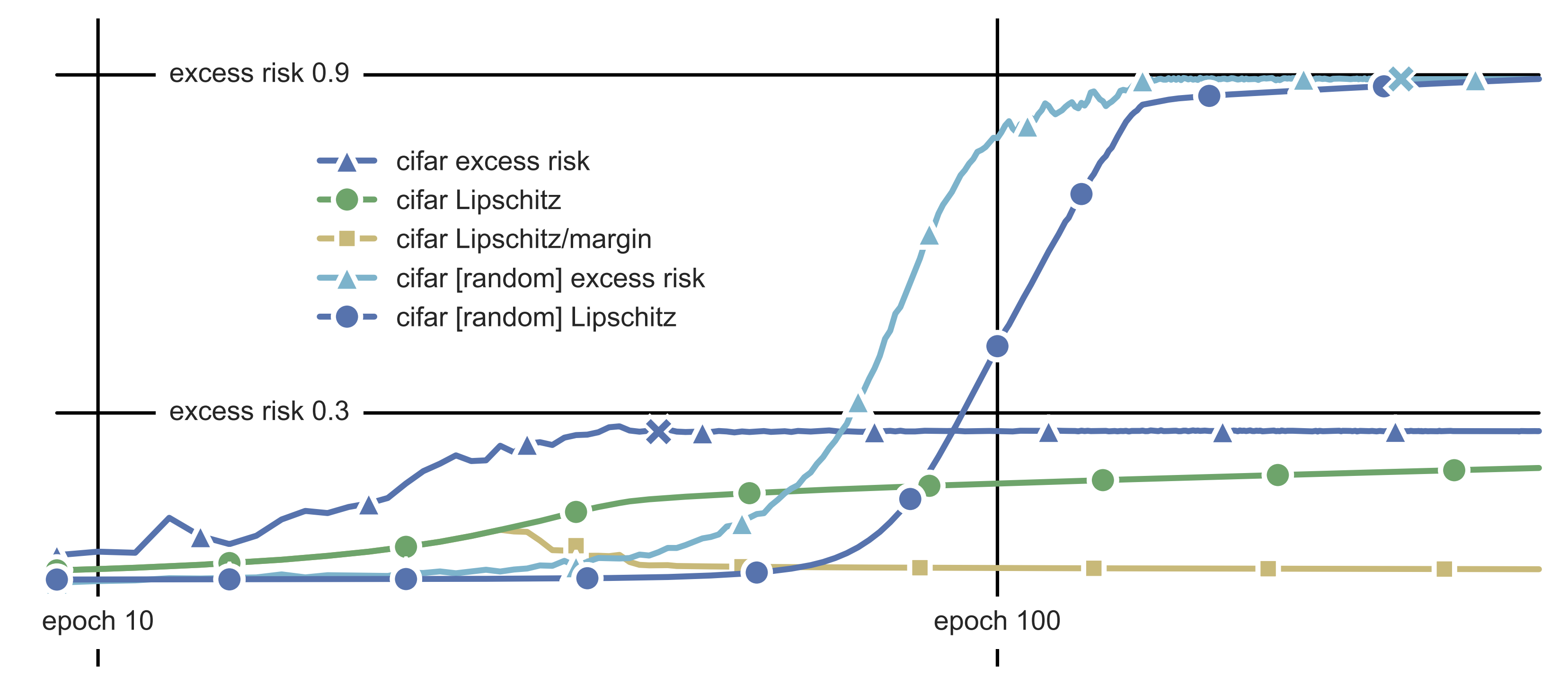
Figure 1. Training AlexNet on CIFAR10 with original or random labels.

The curves track “excess risk” and “Lipschitzness” across epochs. In this figure, excess risk means test error minus training error, the generalization gap, rather than excess population risk over the best function in a class. Crosses mark the first zero-training-error epoch, reached much earlier with original labels. Afterward, the gap equals test error and plateaus near 0.3 for original labels and 0.9 for random labels.

Both networks have the same number of parameters, so parameter count cannot distinguish their substantially different gaps. The complexity curves are lower for original labels and correlate with the observed difference, supporting a more informative complexity measure.

Editorial note: the handout informally identifies the plotted Lipschitz quantity with spectral complexity up to constants. The paper's Lipschitz curves refer to the product of spectral norms; full spectral complexity also includes a mixed-norm correction, which is not generally a fixed constant.

Margin. The unnormalized complexity continues to grow even after the generalization gap plateaus. Thus a bound depending only on $\Vert X{\Vert }_{F}R(W)/n$ does not fully track the behavior. After training error reaches zero, predictions can continue to become more confident as complexity increases.

The prediction is $\arg {\max }_j{f}_W(x{)}_j$, and the margin is

A positive margin guarantees a correct prediction, while a negative margin implies an incorrect one. Larger positive margins indicate greater separation from competing labels. Using the preceding tools and additional standard arguments, the handout states a high-probability bound, simultaneously for networks and $\gamma >0$:

Increasing $\gamma$ increases the empirical small-margin term but decreases the complexity penalty. Simultaneous validity lets the analysis choose the best tradeoff; $\gamma$ need not be a training hyperparameter.

When training error is zero and the minimum margin is positive, taking ${\gamma }_{\min }={\min }_{t}M(f_W,x_t,y_t)$ makes the source's strict-threshold empirical term vanish, leaving the main scale $\Vert X{\Vert }_{F}R(W)/({\gamma }_{\min }n)$. Increasing complexity need not worsen this ratio if margins grow too. The square-marked curve in Figure 1 illustrates the stabilization after margin normalization.

Editorial note: ties can give zero margin even with zero training error. The full probability theorem also has a confidence term, and the original paper uses a different mixed-norm expression. If the empirical indicator uses $M\le \gamma$, take $0<\gamma <{\gamma }_{\min }$ instead. Equation (4) here preserves the handout's leading-order shorthand.

Margin distributions. Normalize margins by $Q=\Vert X{\Vert }_{F}R(W)/n$. For $Q>0$, rescaling the threshold rewrites the leading-order inequality as

The empirical distribution's CDF supplies the first term. The source accidentally writes $\max$ instead of $\arg \max$ in this rewritten probability event; this edition explicitly corrects that typo.

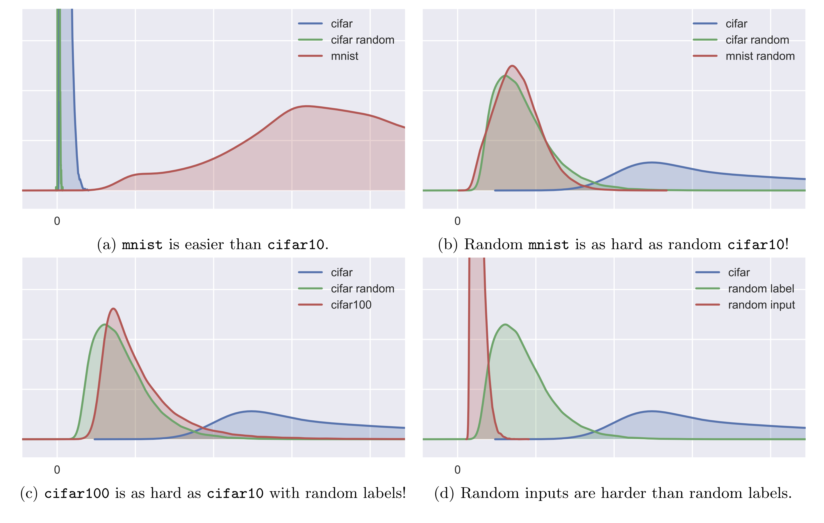
Figure 2. Comparing normalized margin distributions for different tasks.

A distribution placing more mass to the right indicates an easier task under this comparison. The four panels suggest that MNIST is easier than CIFAR10; their randomly labeled versions are similarly difficult; CIFAR100 is nearly as difficult as CIFAR10 with random labels; and random inputs are harder than random labels.

Closing remark. Spectral complexity and margin provide a partial explanation for generalization despite large parameter counts. What remains unexplained is why networks trained on clean data tend to have low complexity. Training is generally not ERM over a class with an explicitly fixed spectral-complexity constraint; it is often a variant of SGD without explicit weight-norm constraints. Understanding the optimization algorithm's implicit preference for low-complexity solutions is a separate nonconvex optimization question.

References

• Peter L. Bartlett, Dylan J. Foster, Matus J. Telgarsky. Spectrally-normalized margin bounds for neural networks. Advances in Neural Information Processing Systems 30, 2017.
• Chiyuan Zhang, Samy Bengio, Moritz Hardt, Benjamin Recht, Oriol Vinyals. Understanding deep learning requires rethinking generalization. International Conference on Learning Representations, 2017.