Based on Haipeng Luo's nine-page Lecture 4, Fall 2026. This report covers Propositions 1–2, Theorems 1–4, Lemmas 1–2, and both figures, explaining motivation, definitions, derivations, and limitations. The scale-sensitive entropy theorem and the full multiclass margin theorem are explicitly identified as external inputs; the remaining key steps are expanded. Added results and corrections are distinguished from the handout. Original: lecture4.pdf (local source, not published online). Companion: full handout reading edition. Prerequisite: Lecture 3. Samples are iid, classes nonempty, and the required measurability and integrability are assumed. Regression functions take values in ; networks here have no biases and use coordinatewise ReLU. Statistical guarantees do not guarantee efficient optimization.
Reading Map: Two Questions Joined by Scale
The first question continues Lecture 3: how can a monotone class be learnable despite infinite pseudo-dimension? Counting arbitrarily small sign changes misses their amplitude. Fat-shattering counts distinctions at a fixed margin.
The second question concerns networks: parameter count need not describe complexity at useful scales. Weight norms yield covering bounds, spectral norms track propagation through layers, and margins compare classification confidence with output scale.
| Sections | Main question | Handout pages |
|---|---|---|
| 1–4 | What does pseudo-dimension miss, and why is the monotone rate ? | 1–2 |
| 5–7 | How does sampling from atoms produce a linear-class cover? | 3–4 |
| 8–10 | Why mixed norms, spectral norms, and recursive error? | 4–6 |
| 11–12 | Where do the exponents and come from? | 6–7 |
| 13–15 | What do margins and the experiments establish? | 7–9 |
| 16–18 | Worked example, pitfalls, and review questions | Throughout |
1. Arbitrarily Small Changes Versus Fixed-Scale Changes
Pseudo-dimension fixes inputs and thresholds, then asks for every sign pattern to be realizable:
It does not distinguish an upward displacement of from one of 0.5. A cover at accuracy 0.01 has no reason to remember the former distinction. Fat-shattering adds a required amplitude:
Positive labels require outputs at least ; negative labels require outputs at most . The two permitted regions are separated by .
The quantifier order matters: fix the points and witness first, vary the entire labeling second, and choose one function for that labeling last. Thresholds cannot depend on labels, and a different function cannot be chosen independently for each coordinate.
Larger scales impose stronger requirements:
For outputs in , no point is shattered if : two outputs realizing opposite labels would need to be more than 2 apart.
With compatible threshold conventions, pseudo-dimension is the supremum over positive-scale fat dimensions. Do not simply substitute into the non-strict inequality: a function equal to every threshold could then appear to realize every labeling, which is not the intended definition.
2. Monotone Functions: Constructions Give Lower Bounds
2.1 Infinite pseudo-dimension
Take , , and prescribe
The worst adjacent labels are , for which
Every pattern therefore extends to a nondecreasing step function on the real line, still in . Any works, but its margin shrinks with .
Requiring restricts this construction to , proving only . Failure of one construction is not an upper bound, because a different construction may exist.
2.2 Why adjacent pairs prove Proposition 1
Suppose some ordered points are shattered with witness . Every adjacent pattern must be realizable, so
Hence adjacent thresholds differ by at least . Different adjacent pairs may use different functions, but they constrain the same witness. Summing gives
This rules out every possible witness and is therefore a genuine upper bound.
2.3 Added result: the exact value in this example
Realizing both labels at every point also forces
Thus , giving . Conversely, whenever , take
All outputs remain in range, and the smallest adjacent increment is zero. A monotone extension exists for every labeling. Therefore
This strengthens the handout's order bound. The constant depends on its convention that the required margin is , rather than .
3. From Fat Dimension to Dudley's Integral
For fixed inputs, define the normalized empirical metric and complexity by
A normalized radius corresponds to Euclidean radius . Theorem 1 is a nontrivial scale-sensitive combinatorial result. A version with safe endpoint constants is
for absolute . The handout does not prove this theorem, and ordinary Sauer counting alone is not a complete proof. We use it as an external input and derive the consequences. Writing also avoids a vanishing logarithm near 1.
Dudley's bound from Lecture 3 is
For the monotone class, the integrand is bounded by a constant times . Substitute :
Letting gives Proposition 2, uniformly over samples. Taking expectation over samples preserves the rate.
The handout uses the simpler estimate . Its integrand is at most a constant times , and
The earlier factor disappears because this covering estimate no longer counts sample locations through a factor.
4. Learnability, Rates, and Loss Assumptions
For a regression loss that is -Lipschitz in the prediction, ERM, symmetrization, and contraction yield
The monotone class consequently has expected excess risk . This is neither zero error on each test point nor a high-probability statement; the latter needs an additional concentration argument and its assumptions.
Even if the entropy integral diverges at zero, finiteness at each positive scale can still establish convergence. Fix . On , fat dimension is bounded by , so the integral is finite. First send , leaving ; then send . Integrability at zero gives a favorable rate, not a necessary condition for convergence.
Necessity must be stated for the relevant real-valued learning model and loss. Lipschitzness alone does not make fat dimension characterize every conceivable loss: the identically zero loss is learnable regardless of the class.
5. The Full Architecture Versus the Trained Network
Fitting random labels shows that the architecture permits a rich class. A vacuous VC upper bound still does not prove that a particular trained predictor generalizes badly on a particular distribution.
Distinguish the full architecture class, a norm-constrained subclass, and the particular predictor selected by optimization. This lecture studies the second object to help explain the third. It does not prove that SGD always selects a low-complexity solution.
For linear predictors, duality and Jensen give a useful warm-up:
Cross terms vanish because distinct Rademacher signs have zero product expectation. If , then , yielding .
No explicit does not mean dimension can never matter. If every input coordinate retains constant scale, the input norm can grow as . Dimension-free statements must be read together with fixed norm bounds.
6. Lemma 1: Sampling a Finite Cover
Here is the proof deferred to HW1, with rounding made explicit. Suppose and
Let equal with probability , and zero with the remaining probability. Then and . For independent draws, define
Independence removes cross terms in the centered error:
Some realization therefore has error at most . Choose . There are at most possible draw sequences, giving
For the metric , set :
If the atoms are sign-symmetric, their convex hull already contains zero and the spare mass can be redistributed. The general formulation includes a zero atom safely. When , the single center zero suffices. When , rounding changes the estimate by at most a factor of 2. Thus the source's principal order is correct, but dropping rounding does not preserve an exact constant of 1.
The mechanism is sparsification: high ambient dimension is tolerable when all vectors have bounded total coefficient mass over a finite atom set. A cover can be indexed by finitely many sampled sequences.
7. Theorem 2: Linear Predictions as Column Atoms
The sample projection is . Omit zero columns and define
Add negative atoms to handle signed coefficients. Cauchy–Schwarz gives
Apply Lemma 1 with , , and at most atoms:
Ignoring universal constants and rounding gives Theorem 2's form. The atom hull only needs to contain the projected class; it need not equal it.
The old bound has mild accuracy dependence. The new bound has mild dimension dependence but an term. Where both are valid, take the smaller one.
8. Theorem 3: Why a Mixed Norm Appears
For , projected outputs form matrices . Use
Coordinatewise ReLU does not expand Euclidean distance. Applying it to both target and cover centers therefore preserves covering accuracy.
Expand
The atom puts feature column into output coordinate , so . After normalization and sign doubling, there are at most atoms. Their coefficient mass is
The mixed norm is exactly what remains after grouping by input column and applying Cauchy–Schwarz. Flattening matrices into coordinates yields, at nontrivial scales,
The denominator's reflects metric normalization, not a guarantee that more outputs make learning easier. With raw Frobenius radius , the denominator becomes simply .
Comparing mixed norms
Let . The triangle inequality gives the complete comparison:
This improves that specific coefficient estimate relative to summing row norms. It does not by itself prove a stronger version of every statement in the original paper.
9. Why Intermediate Centers Must Be Legal Outputs
If , then
This uses both Lipschitzness and . Biases or activations nonzero at the origin require extra terms.
An external cover center need not be a valid intermediate output. To obtain an internal cover, start with external balls of radius . From each ball meeting the set, choose a point in the set. Then
Internal -cover size is consequently bounded by external -cover size. An inverse-square entropy bound incurs a factor of 4; combine this with rounding into a universal constant .
Use for an internal cover at raw Frobenius radius , and set
Each parent center gets its own finite child cover. The norm bound iterates to . Therefore
The union has at most the number of parents times the largest number of children. Taking logarithms turns this into addition. Large-radius cases can use the legal zero output as a single center.
10. Lemma 2: Propagating Error Through Layers
Fix a true network and write , with . Suppose a center satisfies . Choose a child center within of . Then
The matrix norm step follows row by row from , followed by squaring and summing. Set and . Expanding gives
and hence
New error at layer is amplified by later layers. The current spectral norm amplifies preexisting error, which is why the product starts at , not .
If normalized errors were used throughout, the recurrence would instead contain
Working with raw Frobenius errors first avoids silently losing this dimension ratio.
11. Theorem 4: Deriving the 2/3 Allocation
Let the allowed final Frobenius error be , and define
The entropy objective is
Assign final-error shares , with positive summing to one. Then
It remains to minimize . With positive , this objective diverges at the boundary and has positive second derivative , so its unique optimum is interior. The Lagrangian is
Stationarity gives , hence
Set . Substitution yields
Consequently
Replacing with yields the denominator in Theorem 4. Universal constants account for rounding and internal recentering.
A larger makes fine covering more expensive, so the optimum gives that layer a larger share of final error. Its raw local radius can still be smaller because downstream amplification must also be divided out.
12. From Entropy to Spectral Complexity
Define
The squared norm factor in covering entropy becomes . Dudley's square root explains the change from exponent 3 to .
For a precise scalar-output illustration, let , , and assume entropy is at most a constant times over the relevant scales. Let bound the empirical radius. Then
The lower cutoff cannot be zero: this integral diverges. If , choose of that order to obtain
Otherwise, supplies a trivial radius bound. Ignoring logarithms gives , or for bounded input norms.
For vector outputs one must specify the process and final loss. The normalized covering denominator does not automatically give classification an extra improvement. Passing from network covers to a multiclass margin guarantee requires additional empirical-process arguments; scalar contraction alone is not a full proof.
The product of spectral norms bounds Lipschitzness. Full spectral complexity also has a mixed-norm correction. If one weight layer is zero, the bias-free network is identically zero; handle that case separately instead of evaluating a ratio.
13. Margin and Output Scale
For class scores, define
If the true class is 2, scores have margin 1; scores have margin . Zero margin is a tie, whose correctness depends on the tie-breaking rule. Every misclassification lies in .
The ramp loss bridges classification and smooth complexity control:
It is -Lipschitz and satisfies
For a fixed class and threshold, bounded-loss empirical-process theory gives empirical margin loss plus complexity and confidence terms. Uniformity across norm scales and thresholds is an additional step needed before selecting after training.
The handout displays the leading-order relationship
Paper check. The full high-probability theorem also contains a confidence term and uses a row-norm correction, optionally relative to reference matrices. The handout's Equation (4) is a leading-order summary, not a complete numerical probability guarantee. Original Theorem 1.1
Increasing counts more training examples as small-margin but lowers the complexity penalty. A simultaneous bound permits this choice in the analysis without retraining. If all training margins are positive, choose to eliminate the empirical term, regardless of whether an endpoint convention uses or . Zero training error with ties is insufficient.
A homogeneity check
Bias-free ReLU satisfies for . Scaling only the last weight matrix by scales scores and margins by without changing predictions. Mixed-to-spectral norm ratios are unchanged, while their spectral product scales by . Thus
A large raw margin alone is not evidence of better generalization. Rescaling adjacent layers by and preserves both the function and the spectral-complexity expression, another useful check.
14. Figure 1: Identical Parameter Counts, Different Outcomes
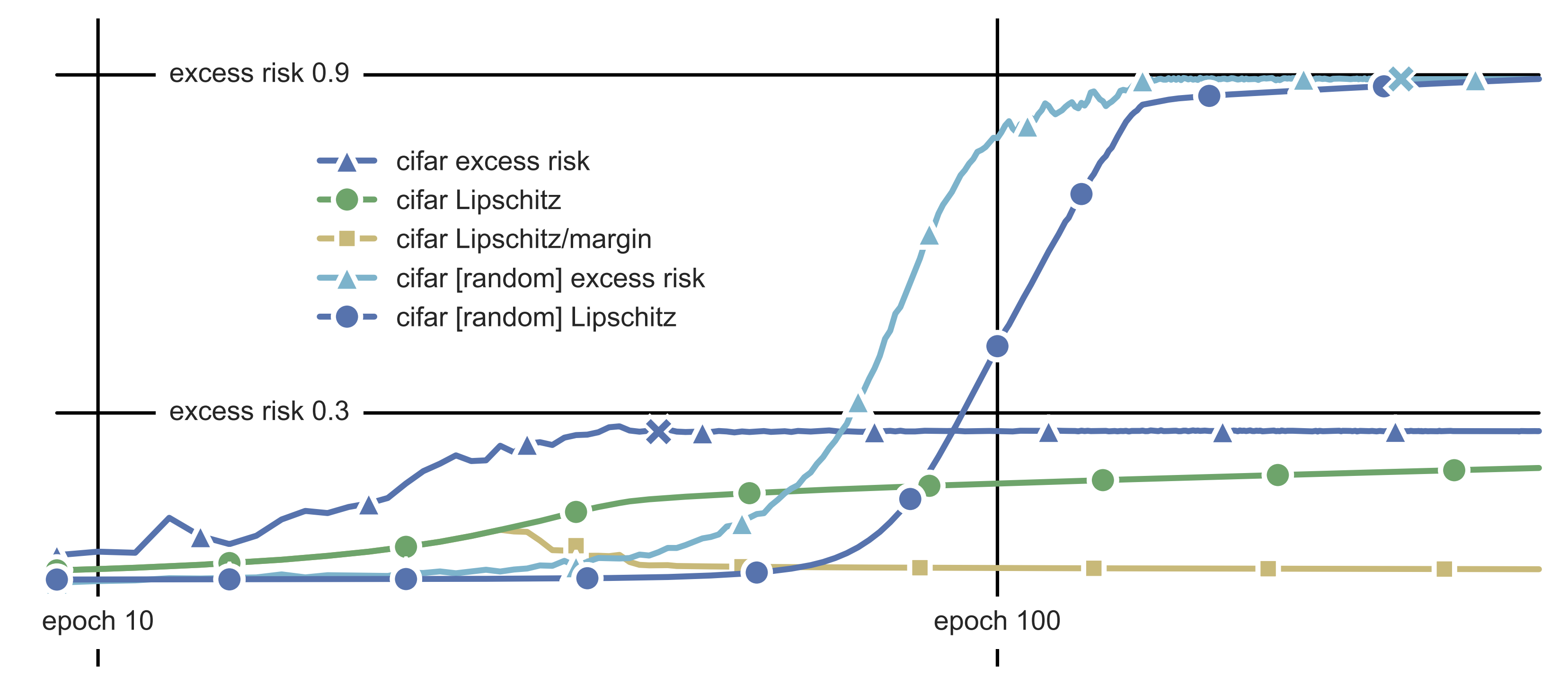
The horizontal axis is training epoch on a logarithmic scale. Crosses mark the first zero-training-error epoch. Here “excess risk” is the test-minus-training error gap, not .
Original labels reach zero training error earlier. Thereafter their test error is about 0.3, compared with about 0.9 for random labels. The parameter counts match, but norm-based curves differ. Error around 0.9 is consistent with ten independently random classes providing no predictive information for new labels.
The unnormalized norm measure can keep growing after the gap stabilizes; dividing by margin can stabilize it. This supports measuring classification relative to output scale. The plotted Lipschitz measure is the spectral-norm product, not automatically the full corrected .
These experiments provide qualitative support in their setting. They do not establish exact prediction of every network's gap, nor guarantee that the bound is numerically below 1.
15. Figure 2: Reading Normalized Margin Distributions
For , write . Rescaling the original threshold to gives leading terms
The first term is the empirical CDF's left limit. The plots show smoothed distribution shapes rather than CDF curves themselves; accumulated mass to the left of a threshold corresponds to the penalty.
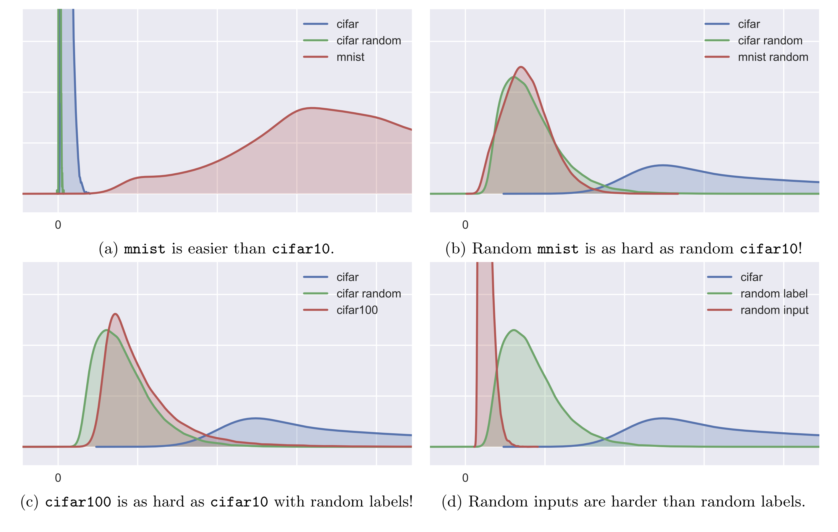
Under comparable normalization, a rightward distribution tends to have less mass below a fixed threshold. More precisely, compare CDFs over relevant thresholds; a larger mean or a shifted peak alone need not suffice.
The panels compare MNIST with CIFAR10, their randomized-label versions, CIFAR100 with randomized CIFAR10, and random inputs with random labels. The indicated ordering is qualitative and specific to those experiments, not an absolute ranking of datasets independent of training.
The handout's rewritten probability formula contains a / typo. Classification error compares a predicted class with a label, not a numerical score with a class index.
16. A Two-Layer Numerical Example
Let , , , and final Frobenius error . Then
Local radii are
Indeed, . Layer 1 has the larger final-error share but the smaller local radius because layer 2 amplifies it.
Dropping common factors, the objective becomes
Equal final-error shares instead give , with objective . The optimized allocation improves the bound.
17. Pitfalls and Source Corrections
| Possible misreading | Correct interpretation |
|---|---|
| Infinite pseudo-dimension forbids learning | Positive-scale fat dimensions retain amplitude information |
| A failed shattering construction proves an upper bound | All possible witnesses must be ruled out |
| Fat dimension is a containing linear subspace's dimension | It controls entropy, not linear containment |
| Every covering radius uses the same normalization | Scalars use , matrices , and the recursion uses raw Frobenius radii |
| Lemma 1 needs neither a zero atom nor rounding | The general sampling statement includes both |
| Recenter a cover without cost | The usual construction doubles the radius |
| Parameter count has no influence whatsoever | Norms and input scale may still depend on dimension |
| Spectral complexity equals Lipschitzness | A mixed-norm correction is also present |
| Zero training error means positive minimum margin | Correctly resolved ties may still have zero margin |
| The plotted excess risk is class-relative excess risk | It is the test-minus-training gap |
| A margin bound proves SGD finds good solutions | It controls certain solutions; selection by optimization is a separate problem |
Handle degenerate cases separately: zero data collapse projections; omit zero columns; a zero layer makes the bias-free network zero; a radius of zero cannot be inserted into an inverse-square bound; and normalized margins are undefined when .
18. Self-Check and Review Order
- Why is monotone pseudo-dimension infinite? Witness thresholds become closer with increasing sample size, so progressively smaller perturbations realize arbitrary signs.
- What is the exact fat dimension at ? Four under the handout's margin convention. Witnesses work.
- Where does inverse-square accuracy come from? Averaging atoms has mean squared error at most .
- Why column followed by ? Group output coefficients by input column, then apply Cauchy–Schwarz against data-column norms.
- Why the exponent? Differentiating gives .
- Can the network entropy integral start at zero? No; its integrand requires a cutoff.
- Does multiplying scores by ten improve classification? Predictions are unchanged, and both margin and spectral complexity scale together.
- What question remains open in the lecture? Why the particular optimizer tends to find low-complexity, favorable-margin solutions.
For a 30-minute review, spend eight minutes reproducing the monotone bounds and integral, seven deriving atom sampling and the mixed norm, ten on the layer recurrence, KKT calculation, and numerical example, and five explaining the figures and the distinction between statistics and optimization.
Sources and Added Material
The primary source is the local Lecture 4 handout, whose numbering is retained. The exact monotone dimension, rounded sampling bound, recentering constants, expanded KKT derivation, homogeneity checks, and numerical example are added derivations. The confidence term and norm conventions were checked against Bartlett, Foster, and Telgarsky (2017). The handout's other reference is Zhang, Bengio, Hardt, Recht, and Vinyals, Understanding deep learning requires rethinking generalization, ICLR 2017.